I have recently written a small pricing library in F# Pricer. It contains a set of methods for derivatives pricing, generating payoff charts, estimating volatility. Payoff charts show you the profit of an option as a function of the share price. This post is about options pricing and the way it can be implemented in F#.

There are generally two methods to price options:

• Black Scholes formula
• Tree based models - binomial or trinomial trees
• Monte carlo methods
• Finite difference methods

Black Scholes is closed-form mathematical formula for pricing European options (options that can be exercised only at the maturity). Binomial pricing is generic method that can be applied to pricing of diverse financial products. All the methods above place the same assumptions on underlying share and it’s movements (which I will describe later)

There are quite a lot of examples of the Black Scholes implementation around the web. Taking into account the fact that it is a mathematical formula, besides translating it into given programming language, there is not that much to talk about. This blog post will be about Binomial Pricing. However, before we got to the code, it’s quite important to understand how the underlying stock movements are modelized.

Share price and it’s movements

In order to determine the price of the option, one has to guess how the shares will move in the future. That is not possible but we can assume two facts:

• the stock price follows a long term direction (in the long term it keeps climbing or it declines)
• the stock oscillates randomly in the short term

These two assumptions are contained in the following equation, which describes the stock movement as generalized Wiener process (type of stochastic process).

let dS = alpha*S*dt + sigma*S*dW

This equation describes the change in the share price (dS) in time (dt), as a function of the current share price (S), the drift (alpha), which is the long term direction of the stock, the volatility (sigma) and (dW) random value, which represents the random swing in the share price in the short time (dt). The volatility affects how big the random swings in the share price will be.

This by it self would not be enough to build any pricing model. A second assumption is based on the share price and it’s daily returns. The daily returns of the stock which follows the generalized Wiener process have log-normal distribution. If we assume, that the daily returns are independent, than the logarithms of daily returns are normally distributed. It is important to keep this assumption in mind. Both methods (BS and Binomial pricing) are based on the fact, that the logs of daily returns are normally distributed and are independent, which in the real time is not the case.

Binomial pricing

The basic idea behind binomial pricing is the following. We assume that the share can move every day up or down, always in the same way. With this knowledge we will build a tree (binomial) which will contain all paths that the share price could undertake from now until certain time in the future (usually the maturity). In the same time, we can construct a second tree which will hold the prices of the derivative. The price of the option depends on the price of the underlying and thus any change in the price of the share will result also in change in the price of the option. Here are the trees:

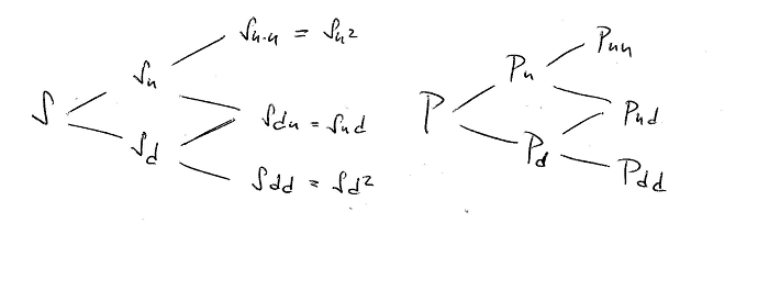
We assume that there are constants u and d which symbolize the movements of the stock. The stock in the next time step will have value S*u if it goes up or S*d if it goes down. So the price of the stock any time in the future in each node can be easily calculated by multiplying by d and u constants. It’s not the case for the derivative tree. We will describe bellow what will be the formula to set the derivative price from the previous nodes.

Delta hedging

Before we come to the formula that explains the derivative price change in the tree, we will have to describe what delta hedging is - the same idea is behind Black & Scholes model as well.

Imagine that we could create a portfolio in which we would hold a certain number of shares (usually called delta) and short position in the derivative (selling the option in the same time) and that we would figure out the exact amount of shares (delta), which would make this portfolio immune to the share price. The portfolio would not loose nor win anything if the share price changes in any way. If we find out the exact number of shares needed to hedge the option, our portfolio should hold a stable value.

So our magic portfolio is:

• long (buy) shares of stock
• short (sell) delta number options - delta S

As said before the price of the option depends on the price of the share. If the price of the derivative changes the following day, because the stock moved, then the delta will change as well, we will have to buy different number of shares to “hedge” the option that we are selling. This practice of continuously adapting to the share and derivative price to keep neutral portfolio is called delta hedging.

Now back to delta, how can we figure out the exact amount of shares to hedge the option?

In a world where there is no arbitrage possible, nor taxes, this portfolio should earn you exactly the neutral interest rate - because it does not move. Taking these assumptions we will try to deduce the delta (the number of shares that we need to hold):

In the equations above:

• delta is the number of shares that we have to hold
• S - is the price of the share now
• P - is the price of the option now
• Su and Pu- the price of the share and option if the stock goes up
• Sd and Pd- the price of the share and option if the stock goes down

We have extracted two pieces of information from the binomial tree:

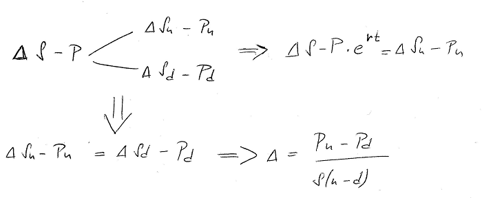
• the value of the portfolio should stay the same, which let’s us solve for delta
• if the stock goes up, then the value of the portfolio should be equal to the portfolio monetized with neutral interest rate.

(delta\*Su - Pu) = (S-P)\*exp(rt)

We will use this knowledge later to determine the price of option P from the prices Pu and Pd in the next nodes. We can use those last two equations and solve for P the price of the option.

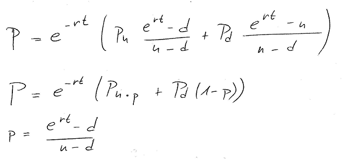
We have defined a technical variable called p (small p) which is usually called technical probability just to simplify the equation, and we have the option price (P) as a function of Pu (the price of the option if the stock goes up) and Pd price of the option if the stock goes down. That means that if we would be able to find the prices of the derivative in the end nodes - at the maturity, we could walk the tree back all the way to the current node, to get the price of the derivative right now.

Now to make the things a bit more complicated, the stocks pay dividends and we have to take that into account. If the dividend yield is q, then the tree of our portfolio would be a bit different:

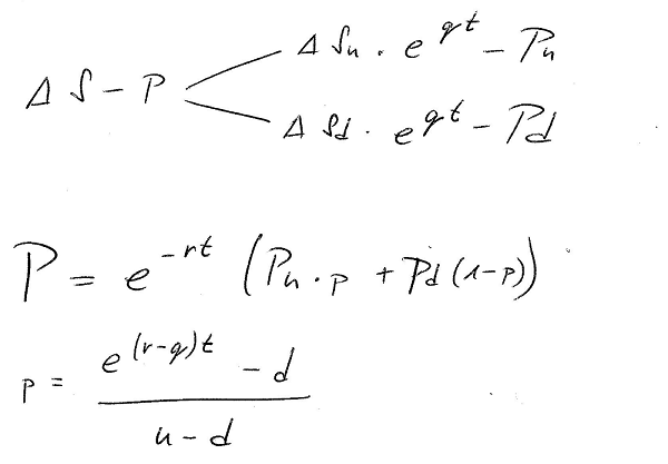
The dividend would raise the price of the stock up a bit in each step top Su*exp(qt), but everything else stays the same. The technical probability (p) now contains the dividend as well.

We have everything, but what we did not yet figured out are the values of u and p the multiplicators which make the stock go up or down.

This was determined by Cox, Ross, & Rubinstein in the CRR binomial pricing model, which tells us to use the volatility to obtain the values of u and d.

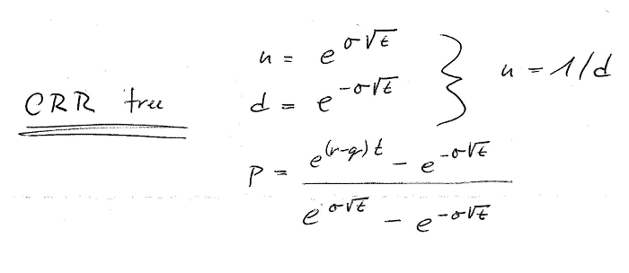
It is beyond the scope of this blog, to explain how this was determined, but note that this is only possible if the log returns of the underlying have normal distribution and if the returns of the stock are independent, (hence that introduction about share price modelization).

Implementation

I will present here two implementations both in F#, the first one is more imperative in style, since it modifies two arrays which represent the actual layer of the binomial tree. The second implementation is purely functional code, however the ratio behind is the same and it is shown on the next images:

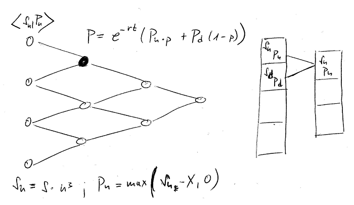
The algorithm has the following steps:

• Determine the prices of the stock and the derivative in the end nodes.
• Go backwards in the tree and compute the price of the derivative (P) as the function of Pu and Pd (derivative prices from the previous nodes)
• In the case of pricing American options, the option can be exercised any time (before maturity). If so, compare in each node the price of the stock to the price of the underlying share, and determine if pre-mature exercise is worth.

The price of the derivative in the end node is calculated with the optionValue function. For call option it would be max(S-X,0) for a put option max(X-S,0), where X is the strike of the option. The following algorithm takes the number of steps in the tree as parameter and an option definition. Option has a property called TimeToExpiry which is the value between the purchase date of the option and the maturity in days. This time is then divided by the number of steps to obtain deltaT the time interval of a single step.

First we will create BinomialContext object which holds all the parameters of our pricing model. There parameters are calculated using the CRR model - that is up and down stock movement is calculated from the volatility, as well as the technical probabilities p_up and p_down.

The technical probability (p) is determined as p_up. We have also defined p_down as 1-(p_up) just to simplify the computations.

let deltaT = option.TimeToExpiry/float steps
let up = exp(stock.Volatility*sqrt deltaT)
let down = 1.0/up
let R = exp (stock.Rate*deltaT)
let p_up = (R-down)/(up-down)
let p_down = 1.0 - p_up

{
    Periods = steps
    Up = up
    Down = down
    PUp = p_up
    PDown = p_down
    Rate = R
    Option = option
    Ref = stock.CurrentPrice
}

This context holds all the setting extracted from our model. It is used by the method that we will describe bellow.

Now we can take a look at the actual iterative implementation. In the first part we prepare our optionValue function which will determine a value on option by looking into the array of stock prices over which we are going to iterate.

We also have to initialize the array to it’s starting values. These are the leaf values in the tree. Remember that we are walking the tree from the lowest layer (further away on the expiry of the option).

// this array holds the prices of the underlying in given period
let prices = Array.zeroCreate ctx.Periods
let option = ctx.Option

// returns a function used to calculate the option prices in the period i.
// it looks into the underlying prices array and compares with strike
let optionValueInPeriod =
    match option.Kind with
            | Call -> fun i -> max 0.0 (prices.[i] - option.Strike)
            | Put -> fun i -> max 0.0 (option.Strike - prices.[i])

// initialize the last price (the underlying wen down * period times)
prices.[0] <- ctx.Ref*(ctx.Down**(float ctx.Periods))
let optionValues = Array.zeroCreate ctx.Periods

optionValues.[0]<- optionValueInPeriod 0
for i in 1 ..ctx.Periods-1 do
    prices.[i] <- prices.[i-1]*ctx.Up*ctx.Up
    optionValues.[i]<- optionValueInPeriod i

Now we can start to walk the array back to the “current time” and update the values. After we finish, the value in the first element will give us the option price “right now”.

let counter = ctx.Periods-2
for step = counter downto 0 do
    for j in 0 .. step do
        optionValues.[j] <- (ctx.PUp*optionValues.[j+1]+ctx.PDown*optionValues.[j])*(1.0/ctx.Rate)
        if option.Style = American then
            prices.[j] <- ctx.Down*prices.[j+1]
            optionValues.[j] <- max optionValues.[j] (optionValueInPeriod j)

buildPricingResult optionValues.[1] optionValues.[0] ctx

Note that the implementation iterates and modifies 2 arrays: optionValues which contains the prices of the derivate and prices which contains the prices of the stock in the current layer.

At the end we construct the result of the pricing (record which holds the Delta and the Premium):

let buildPricingResult previousOptionPrice optionPrice ctx =
    let optionPriceChange = previousOptionPrice - optionPrice
    let underlyingPriceChange = ctx.Ref*ctx.Up - ctx.Ref
    let delta = optionPriceChange / underlyingPriceChange
    {
        Premium = optionPrice
        Delta = delta
    }

The premium is really on the top of our optionValues field. We can also calculate the delta, because we know the price of the option in the previous step as well as the underlying price change.

Functional way

The previous implementation is cool but we iterate over the stock and option price arrays and constantly modify their content, let’s try to come up with an immutable way.

We will need to represent the binomial tree, so we will start with creating the necessary abstractions. As we have said in the reality we keep two trees - tree of the option prices and tree of the underlying prices. We can hold all the information in the same node:

type BinomialNode = {
    Stock: double
    Option: double
    UpParent: BinomialNode option
    DownParent: BinomialNode option
}

Creating a functional implementation can be surprisingly easy, let’s define a function for single step backwards in the tree. This function would take a list of values, which are the values of the nodes in the current layer and produce another list which would contain the derivative prices in the next step. If we pass in a list with 4 items, we should get a list of 3 items, going down until we have only one item, which will be the derivative price.

This is achieved thanks to Seq.pairwise which iterates over all consecutive values in the array - in our case the first item will be P_up and second P_down.

The BinomialContext object will be kept intact, our model does not change, only the implementation does - since this is completely functional way, the context is passed to all the steps as parameter. This is single step up in the tree:

// takes one layer of the binomial tree and generates the next layer
let step pricing optionVal (prices:BinomialNode []) =
    prices
        |> Array.pairwise
        |> Array.map (fun (downNode,upNode) -> mergeNodes downNode upNode optionVal pricing)

So the next question is how we merge the nodes. That is the hard part, but what we really do here is, that we apply the CRR equation, and calculate the option prices in the node from the previous two nodes. The derivative price is the tricky one. The underlying price in the next node is very easy:

let mergeNodes downNode upNode optionVal pricing =

  // calculate the value of the next option, using the CRR
  let derValue = (pricing.PUp * upNode.Option + pricing.PDown * downNode.Option)*(1.0/pricing.Rate)

  // calculate the value of the next stock - simply by raising the old stock
  let stockValue = upNode.Stock * pricing.Down

  // check for premature execution - if it's american option
  let option' =
      match pricing.Option.Style with
          | American ->
              let prematureExValue = optionVal stockValue
              max derValue prematureExValue
          | European -> derValue


  {
      Stock = stockValue
      Option = option'
      UpParent = Some upNode
      DownParent = Some downNode
  }

The last part is to call this tree generation until we have only 1 node in the current layer:

let rec reducePrices prices =
  match prices with
        | [|node|] -> node.Option, node.UpParent.Value.Option
        | prs -> reducePrices (reductionStep prs)

Now one last remark, I am using a method call generateEndNodePrices which gives me the list of the prices in the last nodes. Even this function can be written in nice functional way:

let generateEndNodePrices (ref:float) (up:float) (periods:int) optionVal =
  let down = 1.0 / up
  let lowestStock = ref*(down**(float periods))
  let first = { emptyNode with Stock = lowestStock; Option = optionVal lowestStock}
  let values = Seq.unfold (fun node ->
      let stock' = node.Stock*up*up
      let option' = optionVal stock'
      let nodeBellow = {
          emptyNode with
              Stock = stock'
              Option = option'
      }
      Some (node,nodeBellow)) first
  values |> Seq.take periods |> Seq.toArray

All it takes is to have the share price (ref) and the multiplicator to obtain it’s price in the next step if the price goes up. We can then use unfold to get the price list.